The First-order Integer-valued Autoregressive (INAR(1)) model with zero-inflated (ZI-INAR(1)) and hurdle (H-INAR(1)) innovations is widely used in studying integer-valued time-series data, such as crime count and heatwave frequency. This work implemented the INAR(1) models in Stan.
You can install ZIHINAR1 from GitHub with:
remotes::install_github("fushengyy/ZIHINAR1")Or you can install the released version of ZIHINAR1 from CRAN with:
install.packages("ZIHINAR1")The package contains main function named get_stanfit().
stan_fit <- get_stanfit(mod_type, distri, y, n_pred = 4,
                        thin = 2, chains = 1, iter = 2000, warmup = iter/2,
seed = NA)mod_type: Character string indicating the model
type. Use "zi" for zero-inflated models and
"h" for hurdle models.
distri: Innovation distribution. Options:
"poi": Poisson
"nb": Negative Binomial
"gp": Generalized Poisson (ZI only)
y: A numeric vector of integers representing the
observed data.
n_pred: Integer specifying the number of time points
for future predictions (default is 4).
thin: Integer indicating the thinning interval for
Stan sampling (default is 2).
chains: Integer specifying the number of Markov
chains to run (default is 1).
iter: Integer specifying the total number of
iterations per chain (default is 2000).
warmup: Integer specifying the number of warmup
iterations per chain (default is iter/2).
seed: Numeric seed for reproducibility (default is
NA).
The following are examples showing how to fit the INAR(1) model when data is generated from a zero-inflated Negative Binomial (ZINB) distribution.
library(ZIHINAR1)
y_data <- data_simu(n = 100, alpha = 0.5, rho = 0.3, lambda = 5, disp = 2,
mod_type = "zi", distri = "nb")
stan_fit <- get_stanfit(mod_type = "zi", distri = "nb", y = y_data, n_pred = 5,
iter = 2000, chains = 1, warmup = 500,
thin = 2, seed = 42)
#>
#> SAMPLING FOR MODEL 'anon_model' NOW (CHAIN 1).
#> Chain 1:
#> Chain 1: Gradient evaluation took 0.000715 seconds
#> Chain 1: 1000 transitions using 10 leapfrog steps per transition would take 7.15 seconds.
#> Chain 1: Adjust your expectations accordingly!
#> Chain 1:
#> Chain 1:
#> Chain 1: Iteration: 1 / 2000 [ 0%] (Warmup)
#> Chain 1: Iteration: 200 / 2000 [ 10%] (Warmup)
#> Chain 1: Iteration: 400 / 2000 [ 20%] (Warmup)
#> Chain 1: Iteration: 501 / 2000 [ 25%] (Sampling)
#> Chain 1: Iteration: 700 / 2000 [ 35%] (Sampling)
#> Chain 1: Iteration: 900 / 2000 [ 45%] (Sampling)
#> Chain 1: Iteration: 1100 / 2000 [ 55%] (Sampling)
#> Chain 1: Iteration: 1300 / 2000 [ 65%] (Sampling)
#> Chain 1: Iteration: 1500 / 2000 [ 75%] (Sampling)
#> Chain 1: Iteration: 1700 / 2000 [ 85%] (Sampling)
#> Chain 1: Iteration: 1900 / 2000 [ 95%] (Sampling)
#> Chain 1: Iteration: 2000 / 2000 [100%] (Sampling)
#> Chain 1:
#> Chain 1: Elapsed Time: 3.277 seconds (Warm-up)
#> Chain 1: 9.208 seconds (Sampling)
#> Chain 1: 12.485 seconds (Total)
#> Chain 1:
get_est(distri = "nb", stan_fit = stan_fit)
#> Mean SD Median Q2.5 Q97.5 Rhat
#> alpha 0.5307909 0.04108348 0.5327549 0.44979898 0.6019402 1.0047284
#> rho 0.3696123 0.12017678 0.3837477 0.07870574 0.5645864 1.0047853
#> lambda 4.9954050 0.82387796 5.0098591 3.52989514 6.5890245 0.9998295
#> phi 2.4923431 1.50853128 2.1013737 0.70294059 6.5018753 0.9997752
#> 95%_HPD_Lower 95%_HPD_Upper
#> alpha 0.45032117 0.6028335
#> rho 0.08011943 0.5648035
#> lambda 3.64535329 6.6350831
#> phi 0.48503911 5.3722200
get_mod_sel(y = y_data, mod_type = "zi", distri = "nb", stan_fit = stan_fit)
#> EAIC EBIC DIC WAIC1 WAIC2
#> 1 519.2344 529.6149 527.1945 514.9319 515.2939
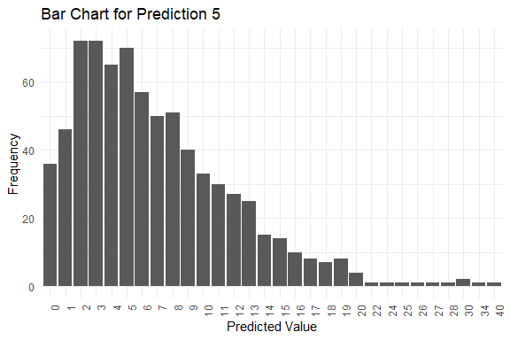
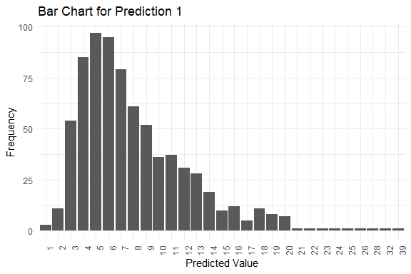
get_pred(stan_fit = stan_fit)
#> $summary
#> Mode Median IQR Min Max
#> y_pred.1 5 7 5 1 39
#> y_pred.2 3 6 7 0 30
#> y_pred.3 4 6 7 0 32
#> y_pred.4 6 6 6 0 28
#> y_pred.5 2 6 7 0 40
#>
#> $plots
#> $plots[[1]]
#>
#> $plots[[2]]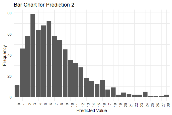
#>
#> $plots[[3]]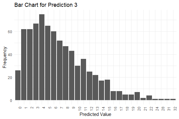
#>
#> $plots[[4]]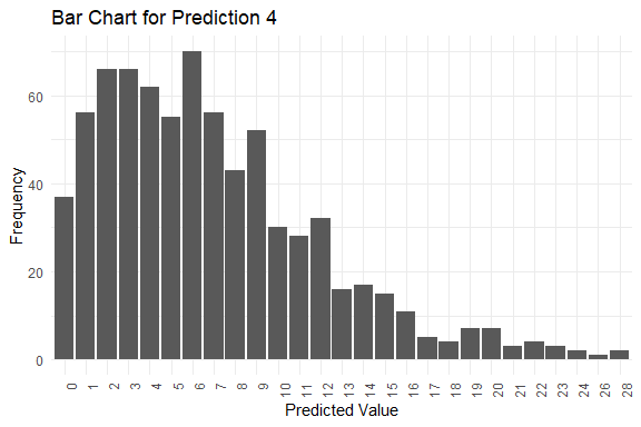
#>
#> $plots[[5]]